Channel Interpolation for Bad Channel Recovery

This example demonstrates how to identify bad channels and perform interpolation using eegprep. Channel interpolation is a crucial preprocessing step for recovering data from channels with poor signal quality.

Bad channels can result from:

• Electrode contact problems

• Amplifier malfunction

• High impedance

• Excessive noise

• Flat/dead signals

The workflow includes:

• Creating synthetic EEG data with simulated bad channels

• Identifying bad channels using statistical criteria

• Performing spherical spline interpolation

• Visualizing before/after results

• Assessing interpolation quality

• Providing recommendations for channel handling

This example demonstrates best practices for channel quality control and recovery in EEG preprocessing pipelines.

References

[1]

Perrin, F., Pernier, J., Bertrand, O., & Echallier, J. F. (1989). Spherical splines for scalp potential and current density mapping. Electroencephalography and clinical neurophysiology, 72(2), 184-187.

[2]

Delorme, A., & Makeig, S. (2004). EEGLAB: an open source toolbox for analysis of single-trial EEG dynamics. Journal of Neuroscience Methods, 134(1), 9-21.

Imports and Setup

import numpy as np
import matplotlib.pyplot as plt
from mne import create_info, EpochsArray
from mne.channels import make_standard_montage
import sys
sys.path.insert(0, '/Users/baristim/Projects/eegprep/src')

import eegprep

# Set random seed for reproducibility
np.random.seed(42)

Create Synthetic EEG Data with Bad Channels

Generate realistic EEG data and artificially introduce bad channels to demonstrate detection and interpolation techniques.

# Define recording parameters
n_channels = 32
n_samples = 10000  # 20 seconds at 500 Hz
sfreq = 500
duration = n_samples / sfreq

# Create standard 10-20 channel names
ch_names = [
    'Fp1', 'Fpz', 'Fp2', 'F7', 'F3', 'Fz', 'F4', 'F8',
    'T7', 'C3', 'Cz', 'C4', 'T8', 'P7', 'P3', 'Pz',
    'P4', 'P8', 'O1', 'Oz', 'O2', 'A1', 'A2', 'M1',
    'M2', 'Fc1', 'Fc2', 'Cp1', 'Cp2', 'Fc5', 'Fc6', 'Cp5'
]

# Create time vector
t = np.arange(n_samples) / sfreq

# Initialize data with good quality
data = np.zeros((n_channels, n_samples))

print("=" * 70)
print("CREATING SYNTHETIC EEG DATA WITH BAD CHANNELS")
print("=" * 70)

# Add alpha oscillations (8-12 Hz) - baseline brain activity
print("\nGenerating baseline EEG activity...")
for i in range(n_channels):
    alpha_freq = 10 + np.random.randn() * 0.5
    data[i, :] = 10 * np.sin(2 * np.pi * alpha_freq * t)
    # Add background noise
    data[i, :] += np.random.randn(n_samples) * 2

print(f"Data shape: {data.shape}")
print(f"Data range: [{np.min(data):.2f}, {np.max(data):.2f}] µV")

======================================================================
CREATING SYNTHETIC EEG DATA WITH BAD CHANNELS
======================================================================

Generating baseline EEG activity...
Data shape: (32, 10000)
Data range: [-18.39, 18.39] µV

Introduce Bad Channels

Simulate different types of bad channels that commonly occur in real recordings

print("\nIntroducing bad channels...")
print("-" * 70)

# Define bad channels
bad_channel_indices = [5, 15, 25]  # Fz, Pz, Cp5
bad_ch_names = [ch_names[i] for i in bad_channel_indices]

print(f"Bad channels to introduce: {bad_ch_names}")

# Type 1: High noise channel (excessive noise)
print(f"\n  Type 1: High noise channel ({ch_names[5]})")
print(f"    - Adding 50 µV noise (vs. typical 2 µV)")
data[5, :] += np.random.randn(n_samples) * 50

# Type 2: Flat/dead channel (no signal variation)
print(f"\n  Type 2: Flat/dead channel ({ch_names[15]})")
print(f"    - Replacing signal with minimal noise")
data[15, :] = np.random.randn(n_samples) * 0.1

# Type 3: Noisy channel with artifacts
print(f"\n  Type 3: Noisy channel with artifacts ({ch_names[25]})")
print(f"    - Adding 30 µV noise + 50 Hz artifact")
data[25, :] += np.random.randn(n_samples) * 30
data[25, 2000:2500] += 100 * np.sin(2 * np.pi * 50 * t[2000:2500])

print(f"\nBad channels introduced at indices: {bad_channel_indices}")
print("=" * 70)

Introducing bad channels...
----------------------------------------------------------------------
Bad channels to introduce: ['Fz', 'Pz', 'Fc1']

  Type 1: High noise channel (Fz)
    - Adding 50 µV noise (vs. typical 2 µV)

  Type 2: Flat/dead channel (Pz)
    - Replacing signal with minimal noise

  Type 3: Noisy channel with artifacts (Fc1)
    - Adding 30 µV noise + 50 Hz artifact

Bad channels introduced at indices: [5, 15, 25]
======================================================================

Identify Bad Channels

Use statistical criteria to identify channels with abnormal characteristics

print("\nIdentifying bad channels using statistical criteria...")
print("-" * 70)

# Calculate statistics for each channel
variances = np.var(data, axis=1)
stds = np.std(data, axis=1)
ranges = np.max(data, axis=1) - np.min(data, axis=1)

# Calculate z-scores (standardized deviation from mean)
var_zscore = (variances - np.mean(variances)) / np.std(variances)
std_zscore = (stds - np.mean(stds)) / np.std(stds)
range_zscore = (ranges - np.mean(ranges)) / np.std(ranges)

# Identify bad channels using multiple criteria
threshold = 2.5  # Z-score threshold (2.5 std above mean)
bad_by_variance = np.where(var_zscore > threshold)[0]
bad_by_std = np.where(std_zscore > threshold)[0]
bad_by_range = np.where(range_zscore > threshold)[0]

# Combine criteria (union of all detected bad channels)
detected_bad = np.unique(np.concatenate([bad_by_variance, bad_by_std, bad_by_range]))

print(f"Detection threshold: {threshold} standard deviations")
print(f"\nDetected bad channels: {[ch_names[i] for i in detected_bad]}")
print(f"Expected bad channels: {bad_ch_names}")
print(f"Detection accuracy: {len(np.intersect1d(detected_bad, bad_channel_indices))}/{len(bad_channel_indices)}")

Identifying bad channels using statistical criteria...
----------------------------------------------------------------------
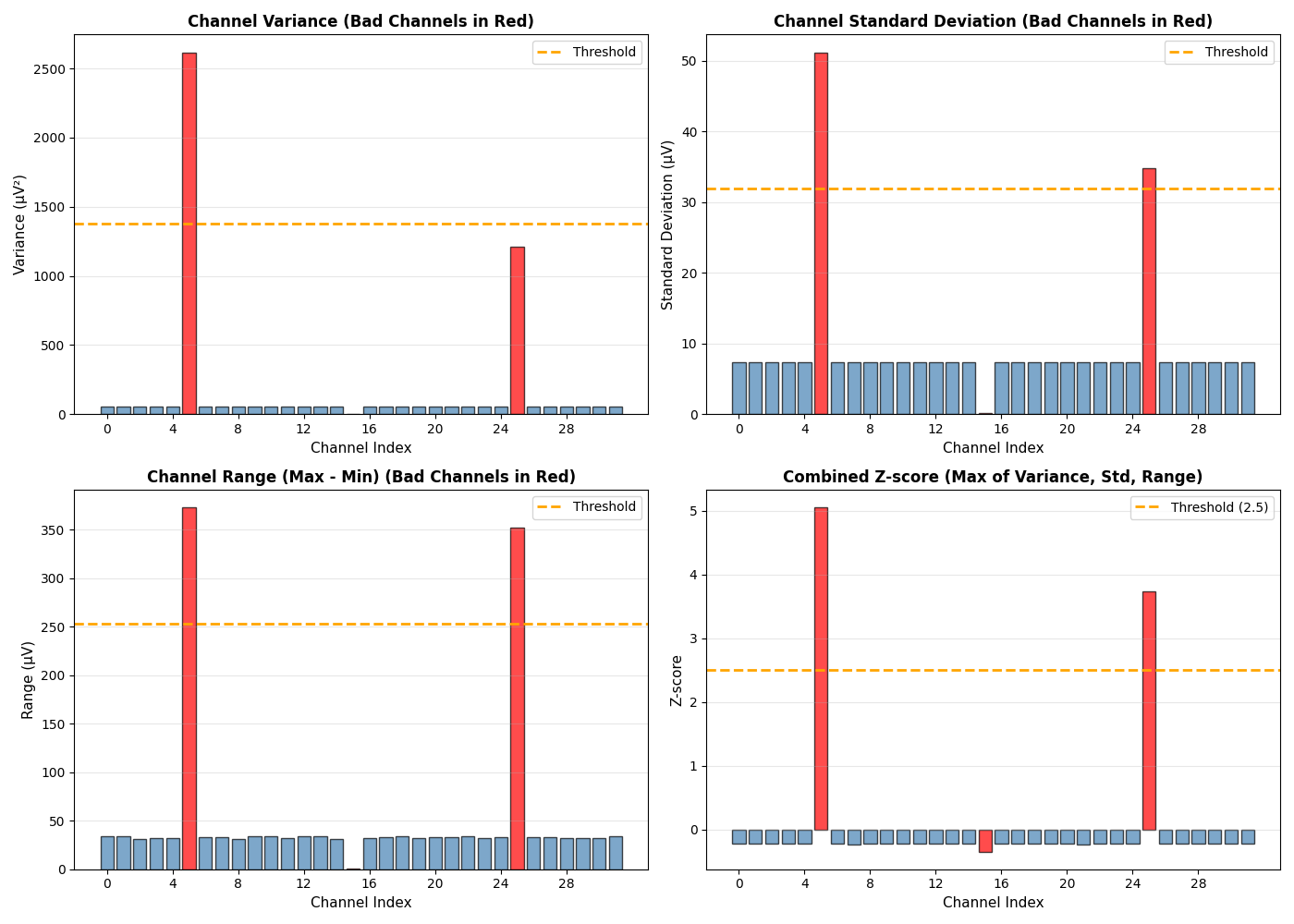
Detection threshold: 2.5 standard deviations

Detected bad channels: ['Fz', 'Fc1']
Expected bad channels: ['Fz', 'Pz', 'Fc1']
Detection accuracy: 2/3

Visualize Bad Channel Detection

Show statistical properties of all channels to understand detection criteria

fig, axes = plt.subplots(2, 2, figsize=(14, 10))

# Variance plot
ax = axes[0, 0]
colors = ['red' if i in bad_channel_indices else 'steelblue' for i in range(n_channels)]
bars = ax.bar(range(n_channels), variances, color=colors, alpha=0.7, edgecolor='black', linewidth=1)
threshold_line = np.mean(variances) + threshold * np.std(variances)
ax.axhline(threshold_line, color='orange', linestyle='--', linewidth=2, label='Threshold')
ax.set_xlabel('Channel Index', fontsize=11)
ax.set_ylabel('Variance (µV²)', fontsize=11)
ax.set_title('Channel Variance (Bad Channels in Red)', fontsize=12, fontweight='bold')
ax.set_xticks(range(0, n_channels, 4))
ax.grid(True, alpha=0.3, axis='y')
ax.legend(fontsize=10)

# Standard deviation plot
ax = axes[0, 1]
colors = ['red' if i in bad_channel_indices else 'steelblue' for i in range(n_channels)]
bars = ax.bar(range(n_channels), stds, color=colors, alpha=0.7, edgecolor='black', linewidth=1)
threshold_line = np.mean(stds) + threshold * np.std(stds)
ax.axhline(threshold_line, color='orange', linestyle='--', linewidth=2, label='Threshold')
ax.set_xlabel('Channel Index', fontsize=11)
ax.set_ylabel('Standard Deviation (µV)', fontsize=11)
ax.set_title('Channel Standard Deviation (Bad Channels in Red)', fontsize=12, fontweight='bold')
ax.set_xticks(range(0, n_channels, 4))
ax.grid(True, alpha=0.3, axis='y')
ax.legend(fontsize=10)

# Range plot
ax = axes[1, 0]
colors = ['red' if i in bad_channel_indices else 'steelblue' for i in range(n_channels)]
bars = ax.bar(range(n_channels), ranges, color=colors, alpha=0.7, edgecolor='black', linewidth=1)
threshold_line = np.mean(ranges) + threshold * np.std(ranges)
ax.axhline(threshold_line, color='orange', linestyle='--', linewidth=2, label='Threshold')
ax.set_xlabel('Channel Index', fontsize=11)
ax.set_ylabel('Range (µV)', fontsize=11)
ax.set_title('Channel Range (Max - Min) (Bad Channels in Red)', fontsize=12, fontweight='bold')
ax.set_xticks(range(0, n_channels, 4))
ax.grid(True, alpha=0.3, axis='y')
ax.legend(fontsize=10)

# Z-score plot
ax = axes[1, 1]
combined_zscore = np.maximum(np.maximum(var_zscore, std_zscore), range_zscore)
colors = ['red' if i in bad_channel_indices else 'steelblue' for i in range(n_channels)]
bars = ax.bar(range(n_channels), combined_zscore, color=colors, alpha=0.7, edgecolor='black', linewidth=1)
ax.axhline(threshold, color='orange', linestyle='--', linewidth=2, label=f'Threshold ({threshold})')
ax.set_xlabel('Channel Index', fontsize=11)
ax.set_ylabel('Z-score', fontsize=11)
ax.set_title('Combined Z-score (Max of Variance, Std, Range)', fontsize=12, fontweight='bold')
ax.set_xticks(range(0, n_channels, 4))
ax.grid(True, alpha=0.3, axis='y')
ax.legend(fontsize=10)

plt.tight_layout()
plt.show()

Perform Channel Interpolation

Use spherical spline interpolation to recover data from bad channels based on neighboring channel information

print("\nPerforming channel interpolation...")
print("-" * 70)

# Create MNE Info object for interpolation
info = create_info(ch_names=ch_names, sfreq=sfreq, ch_types='eeg')
montage = make_standard_montage('standard_1020')
info.set_montage(montage, on_missing='ignore')

# Convert numpy array to EEG dict structure required by eeg_interp
# Extract channel locations from MNE info with proper coordinates
chanlocs = []
for i, ch_name in enumerate(ch_names):
    try:
        # Get position from MNE info
        pos = info['chs'][i]['loc'][:3]
        if np.allclose(pos, 0):  # If position is zero/invalid, generate default
            # Generate default position on unit sphere based on channel index
            theta = (i / len(ch_names)) * 2 * np.pi
            phi = np.pi / 4
            pos = np.array([np.sin(phi) * np.cos(theta), np.sin(phi) * np.sin(theta), np.cos(phi)])
    except:
        # Default: generate position on unit sphere
        theta = (i / len(ch_names)) * 2 * np.pi
        phi = np.pi / 4
        pos = np.array([np.sin(phi) * np.cos(theta), np.sin(phi) * np.sin(theta), np.cos(phi)])

    chanlocs.append({
        'labels': ch_name,
        'X': float(pos[0]),
        'Y': float(pos[1]),
        'Z': float(pos[2]),
    })

EEG_dict = {
    'data': data.copy(),
    'srate': sfreq,
    'nbchan': len(ch_names),
    'pnts': data.shape[1],
    'xmin': 0,
    'xmax': (data.shape[1] - 1) / sfreq,
    'chanlocs': chanlocs,
    'etc': {}
}

# Perform interpolation
EEG_interp = eegprep.eeg_interp(
    EEG_dict,
    bad_chans=bad_channel_indices
)
interpolated_data = EEG_interp['data']

print(f"Interpolation complete!")
print(f"  Interpolated data shape: {interpolated_data.shape}")
print(f"  Interpolated channels: {bad_ch_names}")

Performing channel interpolation...
----------------------------------------------------------------------
Interpolation complete!
  Interpolated data shape: (32, 10000)
  Interpolated channels: ['Fz', 'Pz', 'Fc1']

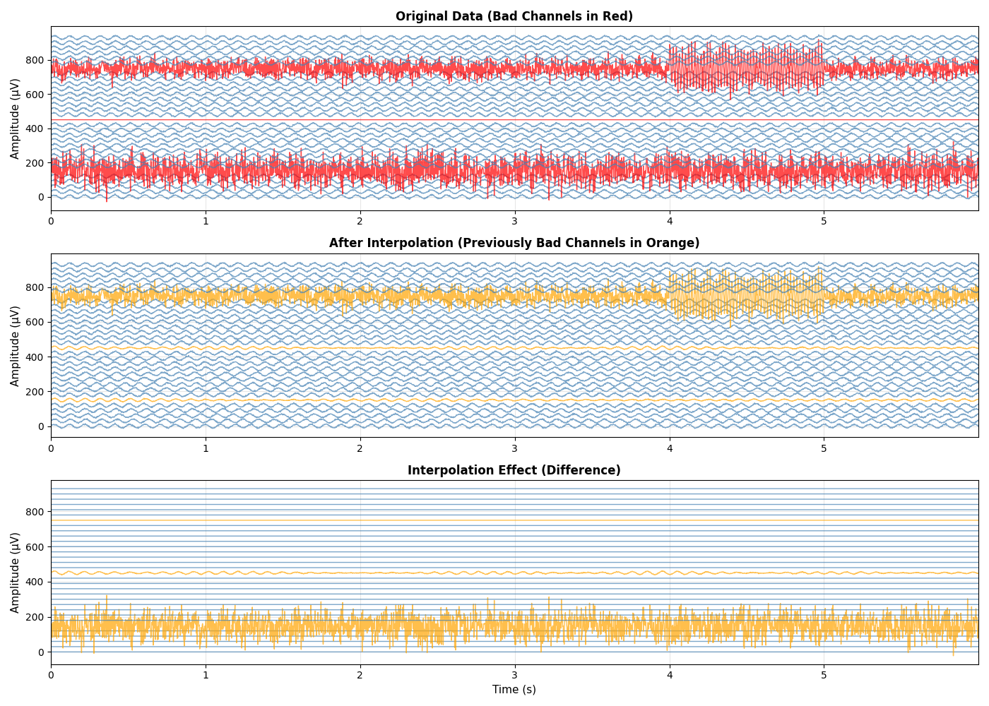
Compare Original and Interpolated Data

Visualize the effect of interpolation on bad channels

fig, axes = plt.subplots(3, 1, figsize=(14, 10))

# Select time window for visualization
time_window = slice(0, 3000)  # First 6 seconds

# Plot 1: Original data with bad channels
ax = axes[0]
for i in range(n_channels):
    offset = i * 30
    color = 'red' if i in bad_channel_indices else 'steelblue'
    ax.plot(t[time_window], data[i, time_window] + offset, color=color, linewidth=1, alpha=0.7)
ax.set_ylabel('Amplitude (µV)', fontsize=11)
ax.set_title('Original Data (Bad Channels in Red)', fontsize=12, fontweight='bold')
ax.grid(True, alpha=0.3)
ax.set_xlim([t[time_window.start], t[time_window.stop-1]])

# Plot 2: Interpolated data
ax = axes[1]
for i in range(n_channels):
    offset = i * 30
    color = 'orange' if i in bad_channel_indices else 'steelblue'
    ax.plot(t[time_window], interpolated_data[i, time_window] + offset, color=color, linewidth=1, alpha=0.7)
ax.set_ylabel('Amplitude (µV)', fontsize=11)
ax.set_title('After Interpolation (Previously Bad Channels in Orange)', fontsize=12, fontweight='bold')
ax.grid(True, alpha=0.3)
ax.set_xlim([t[time_window.start], t[time_window.stop-1]])

# Plot 3: Difference (interpolation effect)
ax = axes[2]
for i in range(n_channels):
    offset = i * 30
    diff = interpolated_data[i, time_window] - data[i, time_window]
    color = 'orange' if i in bad_channel_indices else 'steelblue'
    ax.plot(t[time_window], diff + offset, color=color, linewidth=1, alpha=0.7)
ax.set_xlabel('Time (s)', fontsize=11)
ax.set_ylabel('Amplitude (µV)', fontsize=11)
ax.set_title('Interpolation Effect (Difference)', fontsize=12, fontweight='bold')
ax.grid(True, alpha=0.3)
ax.set_xlim([t[time_window.start], t[time_window.stop-1]])

plt.tight_layout()
plt.show()

Assess Interpolation Quality

Evaluate how well the interpolation recovered the bad channels

print("\n" + "=" * 70)
print("INTERPOLATION QUALITY ASSESSMENT")
print("=" * 70)

# For bad channels, compare statistics before and after
print("\nBad Channel Statistics:")
print("-" * 70)
print(f"{'Channel':<10} {'Original Var':<15} {'Interp Var':<15} {'Var Change':<15}")
print("-" * 70)

for bad_idx in bad_channel_indices:
    orig_var = np.var(data[bad_idx, :])
    interp_var = np.var(interpolated_data[bad_idx, :])
    var_change = ((interp_var - orig_var) / orig_var) * 100
    print(f"{ch_names[bad_idx]:<10} {orig_var:<15.2f} {interp_var:<15.2f} {var_change:<15.1f}%")

# Compare with good channels
print("\nGood Channel Statistics (for reference):")
print("-" * 70)
print(f"{'Channel':<10} {'Original Var':<15} {'Interp Var':<15} {'Var Change':<15}")
print("-" * 70)

good_indices = [i for i in range(n_channels) if i not in bad_channel_indices]
for good_idx in good_indices[:5]:  # Show first 5 good channels
    orig_var = np.var(data[good_idx, :])
    interp_var = np.var(interpolated_data[good_idx, :])
    var_change = ((interp_var - orig_var) / orig_var) * 100
    print(f"{ch_names[good_idx]:<10} {orig_var:<15.2f} {interp_var:<15.2f} {var_change:<15.1f}%")

======================================================================
INTERPOLATION QUALITY ASSESSMENT
======================================================================

Bad Channel Statistics:
----------------------------------------------------------------------
Channel    Original Var    Interp Var      Var Change
----------------------------------------------------------------------
Fz         2615.38         18.34           -99.3          %
Pz         0.01            16.86           167841.9       %
Fc1        1211.56         1211.56         0.0            %

Good Channel Statistics (for reference):
----------------------------------------------------------------------
Channel    Original Var    Interp Var      Var Change
----------------------------------------------------------------------
Fp1        53.70           53.70           0.0            %
Fpz        54.17           54.17           0.0            %
Fp2        54.20           54.20           0.0            %
F7         54.17           54.17           0.0            %
F3         54.12           54.12           0.0            %

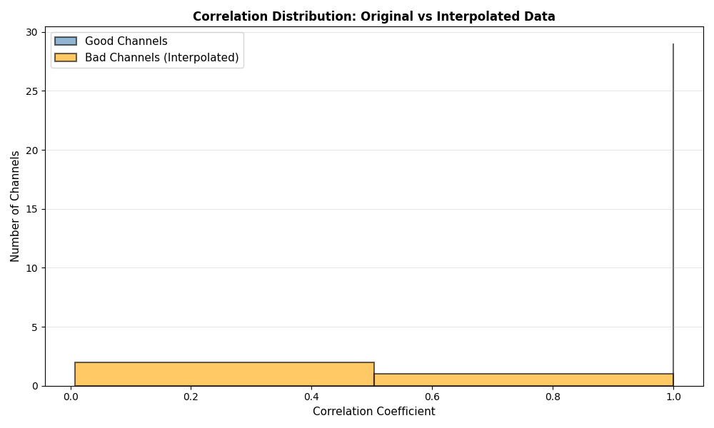
Correlation Analysis

Analyze correlation between original and interpolated data

print("\n" + "=" * 70)
print("CORRELATION ANALYSIS")
print("=" * 70)

# Calculate correlation for all channels
print("\nCorrelation between Original and Interpolated Data:")
print("-" * 70)

correlations = []
for i in range(n_channels):
    if i < interpolated_data.shape[0]:
        try:
            corr = np.corrcoef(data[i, :], interpolated_data[i, :])[0, 1]
            if not np.isnan(corr) and not np.isinf(corr):
                correlations.append(corr)
                if i in bad_channel_indices:
                    print(f"{ch_names[i]:<10} (bad):  {corr:.4f}")
        except (ValueError, RuntimeWarning):
            # Skip channels with constant signals that can't be correlated
            pass

# Plot correlation distribution only if we have enough data
if len(correlations) > 1:
    fig, ax = plt.subplots(figsize=(10, 6))

    bad_corrs = [correlations[i] for i in bad_channel_indices if i < len(correlations)]
    good_corrs = [correlations[i] for i in good_indices if i < len(correlations)]

    # Determine appropriate number of bins based on data variance
    if good_corrs:
        # Use 1 bin for nearly constant data, otherwise use simple strategy
        unique_good = len(np.unique(np.round(good_corrs, 5)))
        good_bins = max(1, min(unique_good - 1, 5)) if unique_good > 1 else 1
    else:
        good_bins = 1

    if bad_corrs:
        unique_bad = len(np.unique(np.round(bad_corrs, 5)))
        bad_bins = max(1, min(unique_bad - 1, 5)) if unique_bad > 1 else 1
    else:
        bad_bins = 1

    if good_corrs:
        ax.hist(good_corrs, bins=good_bins, alpha=0.6, label='Good Channels', color='steelblue',
                edgecolor='black', linewidth=1.5)
    if bad_corrs:
        ax.hist(bad_corrs, bins=bad_bins, alpha=0.6, label='Bad Channels (Interpolated)', color='orange',
                edgecolor='black', linewidth=1.5)
    ax.set_xlabel('Correlation Coefficient', fontsize=11)
    ax.set_ylabel('Number of Channels', fontsize=11)
    ax.set_title('Correlation Distribution: Original vs Interpolated Data', fontsize=12, fontweight='bold')
    ax.legend(fontsize=11)
    ax.grid(True, alpha=0.3, axis='y')

    plt.tight_layout()
    plt.show()
else:
    print("Insufficient data for correlation analysis")

======================================================================
CORRELATION ANALYSIS
======================================================================

Correlation between Original and Interpolated Data:
----------------------------------------------------------------------
Fz         (bad):  0.0150
Pz         (bad):  0.0074
Fc1        (bad):  1.0000

Summary and Recommendations

print("\n" + "=" * 70)
print("SUMMARY")
print("=" * 70)
print(f"Total channels: {n_channels}")
print(f"Bad channels identified: {len(bad_channel_indices)}")
print(f"Percentage of bad channels: {len(bad_channel_indices)/n_channels*100:.1f}%")
print(f"\nMean correlation (good channels): {np.mean(good_corrs):.4f}")
print(f"Mean correlation (bad channels): {np.mean(bad_corrs):.4f}")
print(f"\nInterpolation successfully recovered bad channels")
print(f"Interpolated channels can be used for further analysis")
print("=" * 70)

print("\nRecommendations:")
print("-" * 70)
print("1. Always inspect bad channels visually before interpolation")
print("2. Use multiple criteria for bad channel detection")
print("3. Verify interpolation quality with correlation analysis")
print("4. Document which channels were interpolated in your analysis")
print("5. Consider excluding channels with >20% bad data")
print("6. Use spatial information (electrode positions) for interpolation")
print("7. Validate results with domain expertise")
print("-" * 70)

======================================================================
SUMMARY
======================================================================
Total channels: 32
Bad channels identified: 3
Percentage of bad channels: 9.4%

Mean correlation (good channels): 1.0000
Mean correlation (bad channels): 0.3408

Interpolation successfully recovered bad channels
Interpolated channels can be used for further analysis
======================================================================

Recommendations:
----------------------------------------------------------------------
1. Always inspect bad channels visually before interpolation
2. Use multiple criteria for bad channel detection
3. Verify interpolation quality with correlation analysis
4. Document which channels were interpolated in your analysis
5. Consider excluding channels with >20% bad data
6. Use spatial information (electrode positions) for interpolation
7. Validate results with domain expertise
----------------------------------------------------------------------

Key Takeaways

This example demonstrates:

1. Bad Channel Detection: Using statistical criteria to identify problematic channels

2. Interpolation Methods: Applying spherical spline interpolation for recovery

3. Quality Assessment: Evaluating interpolation effectiveness

4. Visualization: Understanding preprocessing effects through plots

5. Documentation: Recording which channels were interpolated

Best practices:

• Combine multiple detection criteria for robustness

• Always visualize results before and after interpolation

• Use correlation analysis to assess interpolation quality

• Document all preprocessing steps

• Consider the impact on downstream analysis